The skew-normal distribution in JAGS

For a project I'm working on, I decided to try the skew-normal distribution to describe residual noise. JAGS does not have the skew-normal built in, so I used the Bernoulli ones trick to express the skew-normal in a JAGS model specification. This blog post shows how, and also demonstrates that when skew is near zero the autocorrelation can be severe and the posterior distribution has an interesting boomerang shape.

First, an example of simulated data from a skew-normal distribution, along with the recovered parameter values from Bayesian inference.

Gray histogram shows the data; blue curves are a smattering of skew-normals from the posterior.

The generating parameters had values location=1, scale=2, and skew=3. The data had fairly large N=2,000 so that the estimated parameter values might have reasonably high precision. Here are the MCMC diagnostics, along with a pairwise plot of the parameters in the posterior distribution:

These graphs (above) were the result from 12,000 MCMC steps thinned by 5. They have not yet achieved the heuristic desired ESS of 10,000 but at least it's clear that letting the chains run longer would do the job. It's also clear that the data-generating parameter values were recovered fairly well, but interestingly the location is pulled in the direction of the skew, which lets the scale and skew be a bit smaller than their generating values.

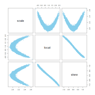
Now another example: The same as before but this time with skew=0, that is, normally distributed data being fit with a skew-normal distribution. In this case, the autocorrelation in the MCMC chains is nasty, and the pairwise posterior distribution shows a boomerang shape:

You can see in the diagnostic plots that the ESS is tiny, despite 12,000 steps thinned by 5. It looks like the chains have settled into the correct parameter values -- after all the posterior-predictive curves superimposed on the data look good -- but it will take a ton more steps to get a smooth representation of the posterior distribution.

Pursuing this topic showed me yet again how Present Self reinvents the wheels of Past Self. I didn't recall ever trying to do this particular application before, so I searched the web to see if anyone had previously posted something about the skew normal distribution in JAGS. One of the first links in the search results was this one, a discussion thread. I skimmed through it and thought it was just the sort of thing I could adapt for my present purposes. I thought the name of the initial poster looked familiar, and then I realized the name of the responder was very familiar -- it was mine. Sigh.

The JAGS model specification, using the Bernoulli ones trick. The Bernoulli ones trick is explained in DBDA2E in Section 8.6.1, pp. 214-215. This script will take several minutes to run for N=2,000; perhaps reduce N on a first try.

# housekeeping
graphics.off() # This closes all of R's graphics windows.
rm(list=ls())  # Careful! This clears all of R's memory!

if ( !("sn" %in% installed.packages()[,"Package"]) ) { install.packages("sn") }
library("sn") 
source("DBDA2E-utilities.R") # for diagMCMC(), openGraph(), etc.!
require(runjags) # should already be loaded from DBDA2E-utilities.R
require(rjags)   # should already be loaded from DBDA2E-utilities.R

# Generate data:

# Specify generating parameter values:
locat = 1 # location
scale = 2 # scale
skew = 3 # skew

# Construct file name root based on generating parameter values:
fileNameRoot = paste0("SkewNormalPlay","-",locat,"-",scale,"-",skew)
saveType = "png"

# Create random data from skew-normal distribution:
N = 2000
set.seed(47405)
y = rsn( N , xi=locat , omega=scale , alpha=skew )
# Scaling constant for use in JAGS Bernoulli ones trick:
dsnMax = 1.1*max(dsn( seq(-10,10,length=1001) , xi=locat,omega=scale,alpha=skew ))
# Assemble data for JAGS:
dataList = list(
  y = y ,
  N = N ,
  ones = rep(1,length(y)) ,
  C = dsnMax # constant for keeping scaled dsn < 1
)

# Define the JAGS model using Bernoulli ones trick
# as explained in DBDA2E Section 8.6.1 pp. 214-215.
modelString = "
model {
  for ( i in 1:N ) {
    dsn[i] <- ( (2/scale) 
                * dnorm( (y[i]-locat)/scale , 0 , 1 ) 
                * pnorm( skew*(y[i]-locat)/scale , 0 , 1 ) )
    spy[i] <- dsn[i] / C
    ones[i] ~ dbern( spy[i] )
  }
  scale ~ dgamma(1.105,0.105)
  locat ~ dnorm(0,1/10^2)
  skew ~ dnorm(0,1/10^2)
}
" # close quote for modelString
writeLines( modelString , con="TEMPmodel.txt" )

# Run the chains:
runJagsOut <- run.jags( method="parallel" ,
                        model="TEMPmodel.txt" , 
                        monitor=c("scale","locat","skew") , 
                        data=dataList ,  
                        #inits=initsList , 
                        n.chains=3 ,
                        adapt=500 ,
                        burnin=500 , 
                        sample=ceiling(12000/3) , 
                        thin=5 ,
                        summarise=FALSE ,
                        plots=FALSE )
codaSamples = as.mcmc.list( runJagsOut ) # from rjags package
save( codaSamples , file=paste0(fileNameRoot,"Mcmc.Rdata") )
mcmcMat = as.matrix( codaSamples )

# Examine the chains:
# Convergence diagnostics:
diagMCMC( codaObject=codaSamples , parName="scale" , 
          saveName=fileNameRoot , saveType=saveType )
diagMCMC( codaObject=codaSamples , parName="locat" , 
          saveName=fileNameRoot , saveType=saveType )
diagMCMC( codaObject=codaSamples , parName="skew" , 
          saveName=fileNameRoot , saveType=saveType )

# Examine correlation of parameters in posterior distribution:
openGraph()
pairs( mcmcMat , col="skyblue" )
saveGraph( file=paste0(fileNameRoot,"-Pairs") , type=saveType )

# plot data with posterior predictions
openGraph(height=4,width=7)
histInfo = hist( dataList$y , probability=TRUE , breaks=31 ,
                 xlab="Data Value" , main="Data with Posterior Pred." ,
                 col="gray" , border="white" )
nCurves = 30
curveIdxVec = round(seq(1,nrow(mcmcMat),length=nCurves))
xComb = seq( min(histInfo$breaks) , max(histInfo$breaks) , length=501 )
for ( curveIdx in curveIdxVec ) {
  lines( xComb , dsn( xComb , 
                      xi=mcmcMat[curveIdx,"locat"] , 
                      omega=mcmcMat[curveIdx,"scale"] , 
                      alpha=mcmcMat[curveIdx,"skew"] ) ,
         col="skyblue" )
}
saveGraph( file=paste0(fileNameRoot,"-Data-PostPred") , type=saveType )

Perhaps this is a case in which Stan would work more efficiently. Read about Stan in Chapter 14 of DBDA2E. Not only would Hamiltonian Monte Carlo drastically reduce autocorrelation, but Stan also has the skew-normal built in. Perhaps a future blog post... if Future Self remembers Present Self...