Monday, December 25, 2017

Which movie is rated better? (Don't treat ordinal ratings as metric)

When deciding what movie to watch online, have you ever considered the star ratings provided by previous viewers? For example, Amazon.com has a 5-star rating system, in which reviewers can give a movie an ordinal rating from 1 star to 5 stars. Here are frequency histograms of 30 movies listed under "drama":

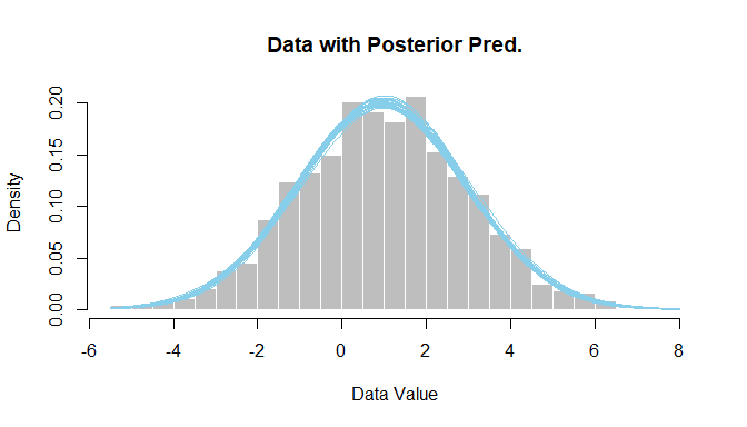
Frequency histograms of star ratings from 30 movies (shown as pink bars). Posterior predictions of an ordered-probit model are shown by blue dots with blue vertical segments indicating the 95% HDIs.

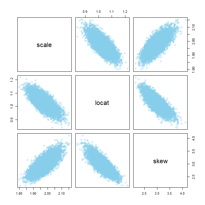
Usually people analyze rating data as if the data were metric, that is, people pretend that 1 star is 1.0 on a metric scale, and 2 stars is 2.0 on the metric scale, and 3 stars is 3.0, and so forth. But this is not appropriate because all we know about the star ratings is their order, not their interval separation. The ordinal data should instead be described with an ordinal model. For more background, see Chapter 23 of DBDA2E, and this manuscript.

Here I used an ordered-probit model to describe the data from the 30 movies. I assumed the same response thresholds across the movies because the response scale is presented to everyone the same way, for all movies; this is a typical assumption. Each movie was given its own latent mean (mu) and standard deviation (sigma). I put no hierarchical structure on the means, as I didn't want the means of small-N movies to be badly shrunken toward enormous-N movies. But I did put hierarchical structure on the standard deviations, because I wanted some constraint on the sigma's of movies that show extreme ceiling effects in their data; it turns out the sigma's were estimated to vary quite a lot anyway.

Below is a graph of the resulting latent means (mu's) of the movies plotted against the means of their ordinal ratings treated as metric:
Each point is a movie. Vertical axis is posterior mean (mu) of ordered probit model, with 95% HDI displayed as blue segment. Horizontal axis is mean of the star ratings treated as metric values.
In the scatter plot above, notice the many non-monotonicities; that is, as the means of ordinal-as-metric values increase along the horizontal axis, the latent mu's do not consistently increase on the vertical axis. In other words, the latent mu's are telling a different story than the ordinal-as-metric means.

Two movies with nearly equal ordinal-as-metric means, but with very different latent means in the ordered-probit model:

Upper row shows ordered-probit fit; lower row shows t test with unequal variances. Notice the blue dots from the ordered-probit model fit the data much better than the blue normal distributions of the ordinal-as-metric model. (Case 19 is Ekaterina: The rise of Catherine the Great, and Case 26 is John Grisham's The Rainmaker.)
Do we conclude that the movies (above) are rated about the same, or that movie 19 is rated much better than movie 26? I think we have to conclude that movie 19 is rated much better than movie 26 because the ordered-probit model is a much better description of the data.

Two movies with ordinal-as-metric means that are significantly different in one direction but the latent means in the ordered-probit model are quite different in the opposite direction:

Upper row shows ordered-probit fit; lower row shows t test with unequal variances. Notice the blue dots from the ordered-probit model fit the data much better than the blue normal distributions of the ordinal-as-metric model. (Case 10 is Miss Sloane, and Case 26 is John Grisham's The Rainmaker.)
Do we conclude that movie 26 is rated better than movie 10, or the other way around? I think we have to conclude that movie 10 is rated better than movie 26 because the ordered probit model is a much better description of the data.

This isn't (only) about movies: The point is that ordinal data from any source should not be treated as metric. Pretending that a rating of "1" is numeric 1.0, and rating "2" is 2.0, and rating "3" is 3.0, and so forth, is usually nonsensical because it's assuming metric information in the data that simply is not there. Treating the data as normally-distributed metric values is often a terrible description of the data. Instead, use an ordinal model for ordinal data. The ordinal model will describe the data better, and sometimes yield rather different implications than the ordinal-as-metric description.

For more information, see Chapter 23 of DBDA2E, and this manuscript titled, "Analyzing ordinal data with metric models: What could possibly go wrong?"

Sunday, December 17, 2017

The skew-normal distribution in JAGS

For a project I'm working on, I decided to try the skew-normal distribution to describe residual noise. JAGS does not have the skew-normal built in, so I used the Bernoulli ones trick to express the skew-normal in a JAGS model specification. This blog post shows how, and also demonstrates that when skew is near zero the autocorrelation can be severe and the posterior distribution has an interesting boomerang shape.

First, an example of simulated data from a skew-normal distribution, along with the recovered parameter values from Bayesian inference.
Gray histogram shows the data; blue curves are a smattering of skew-normals from the posterior.
The generating parameters had values location=1, scale=2, and skew=3. The data had fairly large N=2,000 so that the estimated parameter values might have reasonably high precision. Here are the MCMC diagnostics, along with a pairwise plot of the parameters in the posterior distribution:


These graphs (above) were the result from 12,000 MCMC steps thinned by 5. They have not yet achieved the heuristic desired ESS of 10,000 but at least it's clear that letting the chains run longer would do the job. It's also clear that the data-generating parameter values were recovered fairly well, but interestingly the location is pulled in the direction of the skew, which lets the scale and skew be a bit smaller than their generating values.

Now another example: The same as before but this time with skew=0, that is, normally distributed data being fit with a skew-normal distribution. In this case, the autocorrelation in the MCMC chains is nasty, and the pairwise posterior distribution shows a boomerang shape:


You can see in the diagnostic plots that the ESS is tiny, despite 12,000 steps thinned by 5. It looks like the chains have settled into the correct parameter values -- after all the posterior-predictive curves superimposed on the data look good -- but it will take a ton more steps to get a smooth representation of the posterior distribution.

Pursuing this topic showed me yet again how Present Self reinvents the wheels of Past Self. I didn't recall ever trying to do this particular application before, so I searched the web to see if anyone had previously posted something about the skew normal distribution in JAGS. One of the first links in the search results was this one, a discussion thread. I skimmed through it and thought it was just the sort of thing I could adapt for my present purposes. I thought the name of the initial poster looked familiar, and then I realized the name of the responder was very familiar -- it was mine. Sigh.

The JAGS model specification, using the Bernoulli ones trick. The Bernoulli ones trick is explained in DBDA2E in Section 8.6.1, pp. 214-215. This script will take several minutes to run for N=2,000; perhaps reduce N on a first try.

# housekeeping
graphics.off() # This closes all of R's graphics windows.
rm(list=ls())  # Careful! This clears all of R's memory!

if ( !("sn" %in% installed.packages()[,"Package"]) ) { install.packages("sn") }
library("sn") 
source("DBDA2E-utilities.R") # for diagMCMC(), openGraph(), etc.!
require(runjags) # should already be loaded from DBDA2E-utilities.R
require(rjags)   # should already be loaded from DBDA2E-utilities.R

# Generate data:

# Specify generating parameter values:
locat = 1 # location
scale = 2 # scale
skew = 3 # skew

# Construct file name root based on generating parameter values:
fileNameRoot = paste0("SkewNormalPlay","-",locat,"-",scale,"-",skew)
saveType = "png"

# Create random data from skew-normal distribution:
N = 2000
set.seed(47405)
y = rsn( N , xi=locat , omega=scale , alpha=skew )
# Scaling constant for use in JAGS Bernoulli ones trick:
dsnMax = 1.1*max(dsn( seq(-10,10,length=1001) , xi=locat,omega=scale,alpha=skew ))
# Assemble data for JAGS:
dataList = list(
  y = y ,
  N = N ,
  ones = rep(1,length(y)) ,
  C = dsnMax # constant for keeping scaled dsn < 1
)

# Define the JAGS model using Bernoulli ones trick
# as explained in DBDA2E Section 8.6.1 pp. 214-215.
modelString = "
model {
  for ( i in 1:N ) {
    dsn[i] <- ( (2/scale) 
                * dnorm( (y[i]-locat)/scale , 0 , 1 ) 
                * pnorm( skew*(y[i]-locat)/scale , 0 , 1 ) )
    spy[i] <- dsn[i] / C
    ones[i] ~ dbern( spy[i] )
  }
  scale ~ dgamma(1.105,0.105)
  locat ~ dnorm(0,1/10^2)
  skew ~ dnorm(0,1/10^2)
}
" # close quote for modelString
writeLines( modelString , con="TEMPmodel.txt" )

# Run the chains:
runJagsOut <- run.jags( method="parallel" ,
                        model="TEMPmodel.txt" , 
                        monitor=c("scale","locat","skew") , 
                        data=dataList ,  
                        #inits=initsList , 
                        n.chains=3 ,
                        adapt=500 ,
                        burnin=500 , 
                        sample=ceiling(12000/3) , 
                        thin=5 ,
                        summarise=FALSE ,
                        plots=FALSE )
codaSamples = as.mcmc.list( runJagsOut ) # from rjags package
save( codaSamples , file=paste0(fileNameRoot,"Mcmc.Rdata") )
mcmcMat = as.matrix( codaSamples )

# Examine the chains:
# Convergence diagnostics:
diagMCMC( codaObject=codaSamples , parName="scale" , 
          saveName=fileNameRoot , saveType=saveType )
diagMCMC( codaObject=codaSamples , parName="locat" , 
          saveName=fileNameRoot , saveType=saveType )
diagMCMC( codaObject=codaSamples , parName="skew" , 
          saveName=fileNameRoot , saveType=saveType )

# Examine correlation of parameters in posterior distribution:
openGraph()
pairs( mcmcMat , col="skyblue" )
saveGraph( file=paste0(fileNameRoot,"-Pairs") , type=saveType )

# plot data with posterior predictions
openGraph(height=4,width=7)
histInfo = hist( dataList$y , probability=TRUE , breaks=31 ,
                 xlab="Data Value" , main="Data with Posterior Pred." ,
                 col="gray" , border="white" )
nCurves = 30
curveIdxVec = round(seq(1,nrow(mcmcMat),length=nCurves))
xComb = seq( min(histInfo$breaks) , max(histInfo$breaks) , length=501 )
for ( curveIdx in curveIdxVec ) {
  lines( xComb , dsn( xComb , 
                      xi=mcmcMat[curveIdx,"locat"] , 
                      omega=mcmcMat[curveIdx,"scale"] , 
                      alpha=mcmcMat[curveIdx,"skew"] ) ,
         col="skyblue" )
}
saveGraph( file=paste0(fileNameRoot,"-Data-PostPred") , type=saveType )

Perhaps this is a case in which Stan would work more efficiently. Read about Stan in Chapter 14 of DBDA2E. Not only would Hamiltonian Monte Carlo drastically reduce autocorrelation, but Stan also has the skew-normal built in. Perhaps a future blog post... if Future Self remembers Present Self...

Friday, December 8, 2017

Graphs of imputed censored y values

When using JAGS with censored data, the censored values are imputed to be consistent with the parameters of the model and the censoring limits. It's straight forward to record and graph the imputed values. Here are a couple of slides from my workshops that show how. Start by looking at Section 25.4 of DBDA2E, then the code below follows: