Bayesian estimation supersedes the t test in 15 minutes of video.
For the complete info, see the article and software at this site.
Sunday, November 11, 2012


Friday, October 12, 2012
Abelson's paradox, baseball, null differences, the ROPE, and hierarchical Bayesian analysis
In a thread elsewhere, a reader of Bayesian estimation supersedes the t test commented: "Doesn't Abelson's paradox preclude the establishment of guidelines for a sufficiently small effect size?" In this post I briefly review Abelson's paradox and demonstrate how hierarchical Bayesian data analysis is actually applied to real baseball data of the type that Abelson used to illustrate his paradox. Bayesian estimation provides rich estimates of the abilities of players and their differences. There is no paradox.
First, a cursory review of Abelson's paradox. It was described in a brief article: Abelson, R. P. (1985). A variance explanation paradox: When a little is a lot. Psychological Bulletin, 97(1), 129-133. Abelson considered the batting averages of major league baseball players. A batting average is simply the ratio of number of hits to number of at-bats. In the 2012 season, players each had about 550 opportunities at bat, and typically got about 150 hits, for a typical batting average of about 0.27. Across 143 different players, the batting averages ranged from about 0.19 to 0.34. (Data from ESPN.) Abelson was concerned with whether that variation across players was large compared to the variation within players; in other words, he wanted to know the magnitude of the proportion of variance accounted for by player ability. He came up with a mathematical approximation and argued that for typical data the magnitude of the proportion of variance accounted for is about 0.003. The "paradox" is that such a small number conflicts with sports fans' intuition that player ability should account for a lot more of the variance of hits. Abelson discussed the meaning of his calculation and how it differs from the everyday intuition of the sports fan, saying that his statistic refers to the predictability of a single at-bat. But I can't say I fully understand what Abelson was going for, and the Bayesian analysis of real data (shown below) seems clear and unparadoxical to me.
What does any of that have to do with Bayesian data analysis? Presumably the reader who commented about Abelson's paradox was thinking about the approach to null values that I and others have advocated, whereby a null value for a parameter is deemed accepted for practical purposes if its 95% highest density interval (HDI) falls entirely within a region of practical equivalence (ROPE) around the null value. Perhaps the reader was concerned that no ROPE can be established because even tiny values, like Abelson's 0.003, can correspond to intuitively large effects.
Perhaps the best rebuttal is simply to demonstrate how to do a Bayesian analysis of batting averages, including a ROPE. The analysis uses a hierarchical model that simultaneously estimates individual player abilites and the overall average ability of major league players.
The model comes directly from Chapter 9 of Doing Bayesian Data Analysis. (For an example of applying the same model to meta-analysis of ESP data, see this post. That post also includes a hierarchical diagram of the model.) In the model, the i-th player has an underlying probability of getting a hit, denoted theta[i]. The value of theta[i] is estimated from observing the number of hits y[i] and at-bats N[i] for each player. Importantly, the model assumes that the theta[i] come from a higher-level distribution that describes the individual differences among major league players. There is an overall central tendency, mu, for the batting average of major league players, and a "tightness" of clustering around that central tendency, denoted kappa. (For details, please see Ch. 9 of DBDA.)
The hierarchical structure of the model provides shrinkage in the estimates of the individual abilities. Essentially, each player's data inform the estimate of theta[i] for that player, but also inform the group-level parameters mu and kappa, which in turn influence the estimated values of theta[.] for other players. Thus, if many players all have batting averages right around .27, the group-level distribution is estimated to be very "tight," which pulls in (shrinks) outlying individuals toward the group average. This is intuitively reasonable: If you have information that player after player has an average around .27, you should use that information to inform your estimate of the next player.
When making decisions about differences in estimated abilities, what sort of ROPE is meaningful? There is no single correct answer because it depends on practical consequences. But suppose we say that a difference of 10 hits, in a season of 550 at bats, has practical significance. The ratio 10/550 is just under 0.02, so let's establish a ROPE as -0.02 to +0.02. Our decision rule for assessing differences between players is now this: The difference in abilities between players is deemed to be credibly and practically different from zero if the 95% HDI on the estimated difference falls completely outside a ROPE from -0.20 to +0.02. The difference in abilities is deemed to be practically equivalent to zero if the 95% HDI on the estimated difference falls completely inside the ROPE.
Here are some results from the analysis. First, consider the players with the highest and lowest batting average during the 2012 regular season:
 The right panel shows that their abilities (in terms of estimated probability of getting a hit at bat) are credibly different, and the posterior distribution reveals in detail the relative credibility of the whole range of candidate differences. The graphs also plot the observed batting average (y[i]/N[i]) as small red +'s on the abscissa. Notice that the estimated theta values show clear shrinkage toward the group average. Thus, although Buster Posey had a batting average of 0.336, the estimate of the underlying probability of getting a hit is shrunken toward the major league average, with a mean estimate of 0.313. Similarly, although Carlos Pena had a batting average of 0.197, the estimate of the underlying probability of getting a hit is shrunken toward the central tendency of the group, with a mean estimate of 0.225. Despite the shrinkage, the difference (right panel) is still credibly non-zero.
Here are the results for the two players in the middle of the pack:
 The right panel shows that the estimated difference in their underlying probabilities of getting a hit is nearly zero. 52% of the posterior distribution falls within the ROPE. Thus, we do not have enough precision in the estimate of the differences to declare that their abilities are equal for practical purposes, where "practical" is defined in terms of this choice of ROPE.
Thus, Bayesian analysis provides rich and meaningful inferences about the sort of data that Abelson was interested in. I don't see any "paradox" that needs to be overcome. The Bayesian analysis never even brought up the issue of "proportion of variance accounted for" as Abelson did. Because the Bayesian analysis directly estimates all the parameters of interest, and provides a complete posterior distribution for their credibilities, Abelson's paradoxical statistic never even arose.
Appendix: The complete program. Data are from ESPN, linked in text above.
rm(list = ls())
graphics.off()
fileNameRoot="MajorLeagueBaseballBattingJAGS"
if ( .Platform$OS.type != "windows" ) {
windows <- function( ... ) X11( ... )
}
# In the style of:
require(rjags) # Kruschke, J. K. (2011). Doing Bayesian Data Analysis:
# A Tutorial with R and BUGS. Academic Press / Elsevier.
#------------------------------------------------------------------------------
# THE MODEL.
# Specify the model in JAGS language, but save it as a string in R:
modelString = "
model {
# Likelihood:
for ( i in 1:nPlayers ) {
y[i] ~ dbin( theta[i] , N[i] )
}
# Prior:
for ( i in 1:nPlayers ) {
theta[i] ~ dbeta( a , b )
}
a <- mu * kappa
b <- ( 1.0 - mu ) * kappa
mu ~ dbeta( 1,1 )
kappa ~ dgamma( 1.393 , 0.0393 ) # mode=10, sd=30
}
# ... JAGS model specification ends.
" # close quote to end modelString
# Write the modelString to a file, using R commands:
writeLines(modelString,con="model.txt")
#------------------------------------------------------------------------------
# THE DATA.
dataFrame = read.csv( file="MajorLeagueBaseballBattingStats2012.csv" )
y = dataFrame$H # hits for each player
N = dataFrame$AB # at bats for each player
nPlayers = length(y)
dataList = list(
y = y ,
N = N ,
nPlayers = nPlayers
)
#------------------------------------------------------------------------------
# INTIALIZE THE CHAIN.
# Let JAGS do it randomly...
#------------------------------------------------------------------------------
# RUN THE CHAINS.
parameters = c( "mu" , "kappa" , "theta" ) # The parameter(s) to be monitored.
adaptSteps = 1000 # Number of steps to "tune" the samplers.
burnInSteps = 1000 # Number of steps to "burn-in" the samplers.
nChains = 3 # Number of chains to run.
numSavedSteps=100000 # Total number of steps in chains to save.
thinSteps=1 # Number of steps to "thin" (1=keep every step).
nIter = ceiling( ( numSavedSteps * thinSteps ) / nChains ) # Steps per chain.
# Create, initialize, and adapt the model:
jagsModel = jags.model( "model.txt" , data=dataList , # inits=initsList ,
n.chains=nChains , n.adapt=adaptSteps )
# Burn-in:
cat( "Burning in the MCMC chain...\n" )
update( jagsModel , n.iter=burnInSteps )
# The saved MCMC chain:
cat( "Sampling final MCMC chain...\n" )
codaSamples = coda.samples( jagsModel , variable.names=parameters ,
n.iter=nIter , thin=thinSteps )
# resulting codaSamples object has these indices:
# codaSamples[[ chainIdx ]][ stepIdx , paramIdx ]
#------------------------------------------------------------------------------
# EXAMINE THE RESULTS.
checkConvergence = FALSE
if ( checkConvergence ) {
autocorr.plot( codaSamples , ask=T )
}
# Convert coda-object codaSamples to matrix object for easier handling.
# But note that this concatenates the different chains into one long chain.
# Result is mcmcChain[ stepIdx , paramIdx ]
mcmcChain = as.matrix( codaSamples )
# Extract the posterior sample from JAGS for easier reference:
mu = mcmcChain[,"mu"]
kappa = mcmcChain[,"kappa"] # BRugs gets sample from JAGS
theta = matrix( 0 , nrow=nPlayers , ncol=nChains*nIter )
for ( i in 1:nPlayers ) {
nodeName = paste( "theta[" , i , "]" , sep="" )
theta[i,] = mcmcChain[,nodeName]
}
# Make a graph using R commands:
source("plotPost.R")
windows(width=7,height=2.5)
layout( matrix( 1:2 , nrow=1 , byrow=TRUE ) )
#par(mar=c(2.95,2.95,1.0,0),mgp=c(1.35,0.35,0),oma=c( 0.1, 0.1, 0.1, 0.1) )
plotPost( mu , xlab="mu" , main="Group Mean" )
plotPost( kappa , xlab="kappa" , main="Group Certainty" )
savePlot( file=paste(fileNameRoot,"MuKappa",sep="") , type="jpg" )
plotPlayerDiff = function( idx1 , idx2 , diffRope=c(-0.02,0.02) , savePlotFile=FALSE ) {
windows(width=7,height=2.5)
layout( matrix( 1:3 , nrow=1 , byrow=TRUE ) )
#par(mar=c(2.95,2.95,1.0,0),mgp=c(1.35,0.35,0),oma=c( 0.1, 0.1, 0.1, 0.1) )
plotPost( theta[idx1,] , xlab=paste("theta",idx1) , main=dataFrame$PLAYER[idx1] )
points( dataFrame$AVG[idx1] , 0 , pch="+" , col="red" , cex=1.5 )
plotPost( theta[idx2,] , xlab=paste("theta",idx2) , main=dataFrame$PLAYER[idx2] )
points( dataFrame$AVG[idx2] , 0 , pch="+" , col="red" , cex=1.5)
plotPost( theta[idx1,] - theta[idx2,] ,
xlab=paste("theta",idx1,"-","theta",idx2) , main="Difference" ,
compVal=0.0 , ROPE=diffRope )
points( dataFrame$AVG[idx1]-dataFrame$AVG[idx2] , 0 , pch="+" , col="red" , cex=1.5)
if ( savePlotFile ) {
savePlot( file=paste(fileNameRoot,"Theta",idx1,"Theta",idx2,sep="") , type="jpg" )
}
}
plotPlayerDiff(1,nPlayers,savePlotFile=TRUE)
plotPlayerDiff( round(nPlayers/2)-1 , round(nPlayers/2) ,savePlotFile=TRUE)
First, a cursory review of Abelson's paradox. It was described in a brief article: Abelson, R. P. (1985). A variance explanation paradox: When a little is a lot. Psychological Bulletin, 97(1), 129-133. Abelson considered the batting averages of major league baseball players. A batting average is simply the ratio of number of hits to number of at-bats. In the 2012 season, players each had about 550 opportunities at bat, and typically got about 150 hits, for a typical batting average of about 0.27. Across 143 different players, the batting averages ranged from about 0.19 to 0.34. (Data from ESPN.) Abelson was concerned with whether that variation across players was large compared to the variation within players; in other words, he wanted to know the magnitude of the proportion of variance accounted for by player ability. He came up with a mathematical approximation and argued that for typical data the magnitude of the proportion of variance accounted for is about 0.003. The "paradox" is that such a small number conflicts with sports fans' intuition that player ability should account for a lot more of the variance of hits. Abelson discussed the meaning of his calculation and how it differs from the everyday intuition of the sports fan, saying that his statistic refers to the predictability of a single at-bat. But I can't say I fully understand what Abelson was going for, and the Bayesian analysis of real data (shown below) seems clear and unparadoxical to me.
What does any of that have to do with Bayesian data analysis? Presumably the reader who commented about Abelson's paradox was thinking about the approach to null values that I and others have advocated, whereby a null value for a parameter is deemed accepted for practical purposes if its 95% highest density interval (HDI) falls entirely within a region of practical equivalence (ROPE) around the null value. Perhaps the reader was concerned that no ROPE can be established because even tiny values, like Abelson's 0.003, can correspond to intuitively large effects.
Perhaps the best rebuttal is simply to demonstrate how to do a Bayesian analysis of batting averages, including a ROPE. The analysis uses a hierarchical model that simultaneously estimates individual player abilites and the overall average ability of major league players.
The model comes directly from Chapter 9 of Doing Bayesian Data Analysis. (For an example of applying the same model to meta-analysis of ESP data, see this post. That post also includes a hierarchical diagram of the model.) In the model, the i-th player has an underlying probability of getting a hit, denoted theta[i]. The value of theta[i] is estimated from observing the number of hits y[i] and at-bats N[i] for each player. Importantly, the model assumes that the theta[i] come from a higher-level distribution that describes the individual differences among major league players. There is an overall central tendency, mu, for the batting average of major league players, and a "tightness" of clustering around that central tendency, denoted kappa. (For details, please see Ch. 9 of DBDA.)
The hierarchical structure of the model provides shrinkage in the estimates of the individual abilities. Essentially, each player's data inform the estimate of theta[i] for that player, but also inform the group-level parameters mu and kappa, which in turn influence the estimated values of theta[.] for other players. Thus, if many players all have batting averages right around .27, the group-level distribution is estimated to be very "tight," which pulls in (shrinks) outlying individuals toward the group average. This is intuitively reasonable: If you have information that player after player has an average around .27, you should use that information to inform your estimate of the next player.
When making decisions about differences in estimated abilities, what sort of ROPE is meaningful? There is no single correct answer because it depends on practical consequences. But suppose we say that a difference of 10 hits, in a season of 550 at bats, has practical significance. The ratio 10/550 is just under 0.02, so let's establish a ROPE as -0.02 to +0.02. Our decision rule for assessing differences between players is now this: The difference in abilities between players is deemed to be credibly and practically different from zero if the 95% HDI on the estimated difference falls completely outside a ROPE from -0.20 to +0.02. The difference in abilities is deemed to be practically equivalent to zero if the 95% HDI on the estimated difference falls completely inside the ROPE.
Here are some results from the analysis. First, consider the players with the highest and lowest batting average during the 2012 regular season:

Here are the results for the two players in the middle of the pack:

Thus, Bayesian analysis provides rich and meaningful inferences about the sort of data that Abelson was interested in. I don't see any "paradox" that needs to be overcome. The Bayesian analysis never even brought up the issue of "proportion of variance accounted for" as Abelson did. Because the Bayesian analysis directly estimates all the parameters of interest, and provides a complete posterior distribution for their credibilities, Abelson's paradoxical statistic never even arose.
Appendix: The complete program. Data are from ESPN, linked in text above.
rm(list = ls())
graphics.off()
fileNameRoot="MajorLeagueBaseballBattingJAGS"
if ( .Platform$OS.type != "windows" ) {
windows <- function( ... ) X11( ... )
}
# In the style of:
require(rjags) # Kruschke, J. K. (2011). Doing Bayesian Data Analysis:
# A Tutorial with R and BUGS. Academic Press / Elsevier.
#------------------------------------------------------------------------------
# THE MODEL.
# Specify the model in JAGS language, but save it as a string in R:
modelString = "
model {
# Likelihood:
for ( i in 1:nPlayers ) {
y[i] ~ dbin( theta[i] , N[i] )
}
# Prior:
for ( i in 1:nPlayers ) {
theta[i] ~ dbeta( a , b )
}
a <- mu * kappa
b <- ( 1.0 - mu ) * kappa
mu ~ dbeta( 1,1 )
kappa ~ dgamma( 1.393 , 0.0393 ) # mode=10, sd=30
}
# ... JAGS model specification ends.
" # close quote to end modelString
# Write the modelString to a file, using R commands:
writeLines(modelString,con="model.txt")
#------------------------------------------------------------------------------
# THE DATA.
dataFrame = read.csv( file="MajorLeagueBaseballBattingStats2012.csv" )
y = dataFrame$H # hits for each player
N = dataFrame$AB # at bats for each player
nPlayers = length(y)
dataList = list(
y = y ,
N = N ,
nPlayers = nPlayers
)
#------------------------------------------------------------------------------
# INTIALIZE THE CHAIN.
# Let JAGS do it randomly...
#------------------------------------------------------------------------------
# RUN THE CHAINS.
parameters = c( "mu" , "kappa" , "theta" ) # The parameter(s) to be monitored.
adaptSteps = 1000 # Number of steps to "tune" the samplers.
burnInSteps = 1000 # Number of steps to "burn-in" the samplers.
nChains = 3 # Number of chains to run.
numSavedSteps=100000 # Total number of steps in chains to save.
thinSteps=1 # Number of steps to "thin" (1=keep every step).
nIter = ceiling( ( numSavedSteps * thinSteps ) / nChains ) # Steps per chain.
# Create, initialize, and adapt the model:
jagsModel = jags.model( "model.txt" , data=dataList , # inits=initsList ,
n.chains=nChains , n.adapt=adaptSteps )
# Burn-in:
cat( "Burning in the MCMC chain...\n" )
update( jagsModel , n.iter=burnInSteps )
# The saved MCMC chain:
cat( "Sampling final MCMC chain...\n" )
codaSamples = coda.samples( jagsModel , variable.names=parameters ,
n.iter=nIter , thin=thinSteps )
# resulting codaSamples object has these indices:
# codaSamples[[ chainIdx ]][ stepIdx , paramIdx ]
#------------------------------------------------------------------------------
# EXAMINE THE RESULTS.
checkConvergence = FALSE
if ( checkConvergence ) {
autocorr.plot( codaSamples , ask=T )
}
# Convert coda-object codaSamples to matrix object for easier handling.
# But note that this concatenates the different chains into one long chain.
# Result is mcmcChain[ stepIdx , paramIdx ]
mcmcChain = as.matrix( codaSamples )
# Extract the posterior sample from JAGS for easier reference:
mu = mcmcChain[,"mu"]
kappa = mcmcChain[,"kappa"] # BRugs gets sample from JAGS
theta = matrix( 0 , nrow=nPlayers , ncol=nChains*nIter )
for ( i in 1:nPlayers ) {
nodeName = paste( "theta[" , i , "]" , sep="" )
theta[i,] = mcmcChain[,nodeName]
}
# Make a graph using R commands:
source("plotPost.R")
windows(width=7,height=2.5)
layout( matrix( 1:2 , nrow=1 , byrow=TRUE ) )
#par(mar=c(2.95,2.95,1.0,0),mgp=c(1.35,0.35,0),oma=c( 0.1, 0.1, 0.1, 0.1) )
plotPost( mu , xlab="mu" , main="Group Mean" )
plotPost( kappa , xlab="kappa" , main="Group Certainty" )
savePlot( file=paste(fileNameRoot,"MuKappa",sep="") , type="jpg" )
plotPlayerDiff = function( idx1 , idx2 , diffRope=c(-0.02,0.02) , savePlotFile=FALSE ) {
windows(width=7,height=2.5)
layout( matrix( 1:3 , nrow=1 , byrow=TRUE ) )
#par(mar=c(2.95,2.95,1.0,0),mgp=c(1.35,0.35,0),oma=c( 0.1, 0.1, 0.1, 0.1) )
plotPost( theta[idx1,] , xlab=paste("theta",idx1) , main=dataFrame$PLAYER[idx1] )
points( dataFrame$AVG[idx1] , 0 , pch="+" , col="red" , cex=1.5 )
plotPost( theta[idx2,] , xlab=paste("theta",idx2) , main=dataFrame$PLAYER[idx2] )
points( dataFrame$AVG[idx2] , 0 , pch="+" , col="red" , cex=1.5)
plotPost( theta[idx1,] - theta[idx2,] ,
xlab=paste("theta",idx1,"-","theta",idx2) , main="Difference" ,
compVal=0.0 , ROPE=diffRope )
points( dataFrame$AVG[idx1]-dataFrame$AVG[idx2] , 0 , pch="+" , col="red" , cex=1.5)
if ( savePlotFile ) {
savePlot( file=paste(fileNameRoot,"Theta",idx1,"Theta",idx2,sep="") , type="jpg" )
}
}
plotPlayerDiff(1,nPlayers,savePlotFile=TRUE)
plotPlayerDiff( round(nPlayers/2)-1 , round(nPlayers/2) ,savePlotFile=TRUE)
Tuesday, October 2, 2012
Bayesian estimation of trend with auto-regressive AR(1) deviation
This post is updated here.
This post shows how to estimate trend coefficients when there is an auto-regressive AR(1) process on the deviation from the trend. The specific example uses a sinusoidal trend to describe daily temperatures across many years, but the programming method in JAGS/BUGS can be easily adapted to other trends.
The example extends a previous post about average daily temperatures modeled as sinusoidal variation around a linear trend. The substantive goal was to estimate the slope of the linear component, to determine whether there is a credible non-zero increase in temperatures over the years. In that post, the discussion mentioned lack of independence across days in the deviation from the trend, and with this post the dependence is described by a simple auto-regressive AR(1) model. Here is the model specification with the essential conceptual components highlighted in yellow:
model {
trend[1] <- beta0 + beta1 * x[1] + amp * cos( ( x[1] - thresh ) / wl )
for( i in 2 : Ndata ) {
y[i] ~ dt( mu[i] , tau , nu )
mu[i] <- trend[i] + ar1 * ( y[i-1] - trend[i-1] )
trend[i] <- beta0 + beta1 * x[i] + amp * cos( ( x[i] - thresh ) / wl )
}
ar1 ~ dunif(-1.1,1.1) # or dunif(-0.01,0.01)
beta0 ~ dnorm( 0 , 1.0E-12 )
beta1 ~ dnorm( 0 , 1.0E-12 )
tau ~ dgamma( 0.001 , 0.001 )
amp ~ dunif(0,50)
thresh ~ dunif(-183,183)
nu <- nuMinusOne + 1
nuMinusOne ~ dexp(1/29)
}
The trend is modeled as a linear component plus a sinusoidal component:
trend[i] <- beta0 + beta1 * x[i] + amp * cos( ( x[i] - thresh ) / wl )
The slope on the linear component is beta1.
The predicted value of y at time i, denoted mu[i], is the trend at time i plus a proportion of the deviation from the trend on the previous time step:
mu[i] <- trend[i] + ar1 * ( y[i-1] - trend[i-1] )
Notice that if ar1 is zero, then the model reduces to simply mu[i] = trend[i]. Here is the posterior when ar1 is restricted to being essentially zero, by setting its prior to ar1 ~ dunif(-0.01,0.01):

When ar1 is freely estimated, by setting its prior to ar1 ~ dunif(-1.1,1.1), then the posterior looks like this:

Thursday, September 20, 2012
Workshop on doing Bayesian data analysis at Indiana University

Tuesday, September 18, 2012
From BUGS with BRugs to JAGS with rjags
As mentioned in
several previous posts, I strongly recommend using JAGS instead of BUGS, and I
have converted all the BUGS programs to JAGS versions. Here I provide
guidelines for how to make the conversion in case you want to convert your own
programs.
For a concrete
example, I will use the programs BernTwoBugs.R and BernTwoJags.R. I’ll proceed
section by section through the programs.
The header:
BUGS + BRugs version:
library(BRugs)
JAGS + rjags version:
require(rjags)
Instead of “require”
it could say “library”. Also in the JAGS + rjags version I added a way for the
graphics to work on non-Windows machines. This is just R, so it can work with
BUGS too:
if ( .Platform$OS.type != "windows" ) {
windows <- function(
... ) X11( ... )
}
The model specification:
BUGS + BRugs version:
modelstring = "
# BUGS model specification begins here...
model {
# Likelihood. Each
flip is Bernoulli.
for ( i in 1 : N1 ) {
y1[i] ~ dbern( theta1 ) }
for ( i in 1 : N2 ) {
y2[i] ~ dbern( theta2 ) }
# Prior. Independent
beta distributions.
theta1 ~ dbeta( 3 , 3
)
theta2 ~ dbeta( 3 , 3
)
}
# ... end BUGS model specification
" # close quote for modelstring
# Write model to a file:
.temp = file("model.txt","w") ;
writeLines(modelstring,con=.temp) ; close(.temp)
# Load model file into BRugs and check its syntax:
modelCheck( "model.txt" )
JAGS + rjags version:
modelString = "
# JAGS model specification begins here...
model {
# Likelihood. Each
flip is Bernoulli.
for ( i in 1 : N1 ) {
y1[i] ~ dbern( theta1 ) }
for ( i in 1 : N2 ) {
y2[i] ~ dbern( theta2 ) }
# Prior. Independent
beta distributions.
theta1 ~ dbeta( 3 , 3
)
theta2 ~ dbeta( 3 , 3
)
}
# ... end JAGS model specification
" # close quote for modelstring
# Write the modelString to a file, using R commands:
writeLines(modelString,con="model.txt")
Notice that the
model specification is the same in JAGS as in BUGS. Also, in both cases the
modelString gets written to a file called “model.txt”. The JAGS + rjags version
uses a streamlined version of writeLines that would also work in the BUGS
program, as it is just an R command. The only difference is in how the
specification gets communicated to BUGS or JAGS: BRugs uses the modelCheck
command, but there is no analogous command in rjags.
The data:
BUGS + BRugs version:
# Specify the data in a form that is compatible with BRugs
model, as a list:
datalist = list(
N1 = 7 ,
y1 = c( 1,1,1,1,1,0,0
) ,
N2 = 7 ,
y2 = c( 1,1,0,0,0,0,0
)
)
# Get the data into BRugs:
modelData( bugsData( datalist ) )
JAGS + rjags version:
# Specify the data in a form that is compatible with JAGS model,
as a list:
dataList = list(
N1 = 7 ,
y1 = c( 1,1,1,1,1,0,0
) ,
N2 = 7 ,
y2 = c( 1,1,0,0,0,0,0
)
)
The
specification of the data is the same in JAGS as in BUGS. The only difference
is in how the specification gets communicated to BUGS or JAGS.: BRugs uses the modelData
command, but there is no analogous command in rjags.
Initialize the chains:
BUGS + BRugs version:
modelCompile()
modelGenInits()
JAGS + rjags version:
# Can be done automatically in jags.model() by commenting out
inits argument.
# Otherwise could be established as:
# initsList = list( theta1 =
sum(dataList$y1)/length(dataList$y1) ,
# theta2
= sum(dataList$y2)/length(dataList$y2) )
The BUGS
version has to compile the model (using the BRugs modelCompile command) and
then generate initial values (using the BRugs modelGenInits command). The JAGS
version does not need any explicit initialization at this point, as the
commented code explains.
Run the chains:
BUGS + BRugs version:
samplesSet( c( "theta1" , "theta2" ) ) #
Keep a record of sampled "theta" values
chainlength = 10000 # Arbitrary length of
chain to generate.
modelUpdate( chainlength ) # Actually generate the chain.
JAGS + rjags version:
parameters = c( "theta1" , "theta2" ) # The parameter(s) to be monitored.
adaptSteps = 500
# Number of steps to "tune" the samplers.
burnInSteps = 1000
# Number of steps to "burn-in" the samplers.
nChains = 3
# Number of chains to run.
numSavedSteps=50000
# Total number of steps in chains to save.
thinSteps=1
# Number of steps to "thin" (1=keep every step).
nIter = ceiling( ( numSavedSteps * thinSteps ) / nChains ) #
Steps per chain.
# Create, initialize, and adapt the model:
jagsModel = jags.model( "model.txt" , data=dataList ,
# inits=initsList ,
n.chains=nChains , n.adapt=adaptSteps )
# Burn-in:
cat( "Burning in the MCMC chain...\n" )
update( jagsModel , n.iter=burnInSteps )
# The saved MCMC chain:
cat( "Sampling final MCMC chain...\n" )
codaSamples = coda.samples( jagsModel ,
variable.names=parameters ,
n.iter=nIter , thin=thinSteps )
# resulting codaSamples object has these indices:
# codaSamples[[ chainIdx
]][ stepIdx , paramIdx ]
Roughly the
equivalent of BRugs modelCompile is rjags jags.model. For burning in, the rough
equivalent of BRugs modelUpdate before samplesSet is rjags update. Notice that the BUGS version
here did no burning in. For the final chain, the rough equivalent of BRugs
modelUpdate is rjags coda.samples. Notice that rjags specifies the parameters
to be stored with the variable.names argument in the coda.samples command,
whereas BRugs specifies the parameters in its samplesSet command.
Examine the results:
BUGS + BRugs version:
theta1Sample = samplesSample( "theta1" ) # Put sampled
values in a vector.
theta2Sample = samplesSample( "theta2" ) # Put sampled
values in a vector.
# Plot the trajectory of the last 500 sampled values.
…
JAGS + rjags version:
# Convert coda-object codaSamples to matrix object for easier
handling.
# But note that this concatenates the different chains into one
long chain.
# Result is mcmcChain[ stepIdx , paramIdx ]
mcmcChain = as.matrix( codaSamples )
theta1Sample = mcmcChain[,"theta1"] # Put sampled
values in a vector.
theta2Sample = mcmcChain[,"theta2"] # Put sampled
values in a vector.
# Plot the trajectory of the last 500 sampled values.
…
Once the chain
is put into variables in R, they can be plotted the same way.
One big
difference not shown above is how the chains can be examined for
autocorrelation and convergence. My homegrown plotChains function uses BRugs
commands and will not work with the JAGS output. Instead, JAGS+rjags returns
the chain as a coda-package object, named codaSamples above. There are many
useful functions in the coda package for displaying the chains, not shown
above. For example, summary( codaSamples ), plot( codaSamples ), and autocorr.plot(
codaSamples ).
Thursday, September 6, 2012
Posterior predictive check can and should be Bayesian
 |
| Perception apparently employs prior knowledge that illumination comes from above, and that the surface itself has constant color. |
Abstract: Bayesian inference is conditional on the space of models assumed by the analyst. The posterior distribution indicates only which of the available parameter values are less bad than the others, without indicating whether the best available parameter values really fit the data well. A posterior predictive check is important to assess whether the posterior predictions of the least bad parameters are discrepant from the actual data in systematic ways. Gelman and Shalizi (2012a) assert that the posterior predictive check, whether done qualitatively or quantitatively, is non-Bayesian. I suggest that the qualitative posterior predictive check might be Bayesian, and the quantitative posterior predictive check should be Bayesian. In particular, I show that the “Bayesian p value,” from which an analyst attempts to reject a model without recourse to an alternative model, is ambiguous and inconclusive. Instead, the posterior predictive check, whether qualitative or quantitative, should be consummated with Bayesian estimation of an expanded model. The conclusion agrees with Gelman and Shalizi (2012a) regarding the importance of the posterior predictive check for breaking out of an initially assumed space of models. Philosophically, the conclusion allows the liberation to be completely Bayesian instead of relying on a non-Bayesian deus ex machina. Practically, the conclusion cautions against use of the Bayesian p value in favor of direct model expansion and Bayesian evaluation.Kruschke, J. K. (in press). Posterior predictive check can and should be Bayesian: Comment on Gelman and Shalizi (2012a). British Journal of Mathematical and Statistical Psychology.
Get the full manuscript here.
Monday, September 3, 2012
One-group version of BEST (Bayesian estimation supersedes the t test)
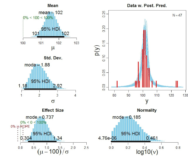
The in-press article, Bayesian estimation supersedes the t test, focuses on the two-group case. Various readers have wanted a one-group version, which is now available. It is in the zip file with the two-group programs.
Here is an example of the code for using the program:
# Specify the data
y = c(101,100,102,104,102,97,105,105,98,101,100,123,105,103,100,95,102,106,
109,102,82,102,100,102,102,101,102,102,103,103,97,97,103,101,97,104,
96,103,124,101,101,100,101,101,104,100,101)
# Run the Bayesian analysis:
source("BEST1G.R")
mcmcChain = BEST1Gmcmc( y )
# Display the results:
BEST1Gplot( y , mcmcChain , compValm=100 , ROPEeff=c(-0.1,0.1) , pairsPlot=TRUE )
The function BEST1Gplot returns detailed numerical summaries of the posterior distribution (not shown here), and it also produces graphical output like this:

Here is an example of the code for using the program:
# Specify the data
y = c(101,100,102,104,102,97,105,105,98,101,100,123,105,103,100,95,102,106,
109,102,82,102,100,102,102,101,102,102,103,103,97,97,103,101,97,104,
96,103,124,101,101,100,101,101,104,100,101)
# Run the Bayesian analysis:
source("BEST1G.R")
mcmcChain = BEST1Gmcmc( y )
# Display the results:
BEST1Gplot( y , mcmcChain , compValm=100 , ROPEeff=c(-0.1,0.1) , pairsPlot=TRUE )
The function BEST1Gplot returns detailed numerical summaries of the posterior distribution (not shown here), and it also produces graphical output like this:


Subscribe to:
Posts (Atom)