Thursday, February 16, 2017

Equivalence testing (two one-sided test) and NHST compared with HDI and ROPE


In this blog post I show that frequentist equivalence testing (using the procedure of two one-sided tests: TOST) with null hypothesis significance testing (NHST) can produce conflicting decisions for the same parameter values, that is, TOST can accept the value while NHST rejects the same value. The Bayesian procedure using highest density interval (HDI) with region of practical equivalence (ROPE) never produces that conflict.

The Bayesian HDI+ROPE decision rule.

For a review of the HDI+ROPE decision rule, see this blog post and specifically this picture in that blog post. To summarize:
  • A parameter value is rejected when its ROPE falls entirely outside the (95%) HDI. To "reject" a parameter value merely means that all the most credible parameter values are not practically equivalent to the rejected value. For a parameter value to be "rejected", it is not merely outside the HDI!
  • A parameter value is accepted when its ROPE completely contains the (95%) HDI. To "accept" a parameter value merely means that all the most credible parameter values are practically equivalent to the accepted value. For a parameter value to be "accepted", it is not merely inside the HDI! In fact, parameter values can be "accepted" that are outside the HDI, because reject or accept depends on the ROPE.
The frequentist TOST procedure for equivalence testing.

In the frequentist TOST procedure, the analyst sets up a ROPE, and does a one-sided test for being below the high limit of the ROPE and another one-sided test for being above the low limit of the ROPE. If both limits are rejected, the parameter value is "accepted". The TOST is the same as checking that the 90% (not 95%) confidence interval falls inside the ROPE. The TOST procedure is used to decide on equivalence to a ROPE'd parameter value.

To reject a parameter value, the frequentist uses good ol' NHST. In other words, if the parameter value falls outside the 95% CI, it is rejected.

Examples comparing TOST+NHST with HDI+ROPE.

Examples below show the ranges of parameter values rejected, accepted, undecided, or conflicting (both rejected and accepted) by the two procedures.
  • In these cases the ROPE is symmetric around its parameter value, with ROPE limits at \(-0.1\) and \(+0.1\) the central value. These are merely default ROPE limits we might use if the parameter value were the effect-size Cohen's \(\delta\) because \(0.1\) is half of a "small" effect size. In general, ROPE limits could be asymmetric, and should be chosen in the context of current theory and measurement abilities. The key point is that the ROPE is the same for TOST and for HDI procedures for all the examples.
  • In all the examples, the 95% HDI and the 95% CI are arbitrarily set to be equal. In general, the 95% HDI and 95% CI will not be equal, especially when the CI is corrected for multiple tests or correctly computed for stopping rules that do not assume fixed sample size. But merely for simplicity of comparison, the 95% HDI and 95% CI are arbitrarily set equal to each other. The 90% CI is set to 0.83 times the width of the 95% CI, as it would be for a normal distribution. The exact numerical value does not matter for the qualitative results.
For each example, plots show the parameter values that would be accepted, rejected, undecided, or conflicting: both accepted and rejected. The horizontal axis is the parameter value. The horizontal black bars indicate the CI or HDI. The vertical axis indicates the different decisions.

Example 1: HDI and 90% CI are wider than the ROPE.

In the first example below, the HDI and 90% CI are wider than the ROPE. Therefore no parameter values can be accepted, because the ROPE, no matter what parameter value it is centered on, can never contain the HDI or 90% CI.
Example 1.
Notice above that NHST rejects all parameter values outside the 95% CI, whereas the HDI+ROPE procedure only rejects parameter values that are a half-ROPE away from the 95% HDI. All other parameter values are undecided (neither rejected nor accepted).

Example 2: HDI and 90% CI are a little narrower than the ROPE.

In the next example, below, the HDI and 90% CI are a little narrower than the ROPE. Therefore there are some parameter values which have ROPE's that contain the HDI or 90% CI and are "accepted". Notice that the TOST procedure accepts a wider range of parameter values than the HDI+ROPE decision rule, because the 90% CI is narrower than the 95% HDI (which in these examples is arbitrarily set equal to the 95% CI).
Example 2.
Notice above that qualitatively the TOST procedure for equivalence produces qualitatively similar results to the HDI+ROPE decision rule, but the TOST procedure accepts a wider range of parameter values because its 90% CI is narrower (i.e., less conservative) than the 95% HDI.

Example 3: HDI and 90% CI are much narrower than the ROPE.

The third example, below, had the HDI and CI considerably narrower than the ROPE. This situation might arise when there is a windfall of data, with high precision estimates but lenient tolerance for "practical equivalence". Notice that this leads to conflicting decisions for TOST and NHST: There are parameter values that are both accepted by TOST by rejected by NHST. Conflicts like this cannot happen when using the HDI+ROPE decision rule.

Example 3
Notice above that some parameter values are "accepted" for practical purposes even though they fall outside the HDI or CI. This points out the very different meaning of the discrete decision and the HDI or CI. The Bayesian HDI marks the most credible parameter values, but the green "accept" interval marks all the parameter values to which the most credible values are practically equivalent. The frequentist CI marks the parameter values that would not be rejected, but the green "accept" interval marks all the parameter values that pass the TOST procedure.

The comparison illustrated here was inspired by a recent blog post by Daniel Lakens, which emphasized the similarity of results using TOST and HDI+ROPE. Here I've tried to illustrate at least one aspect of their different meanings.

Wednesday, February 8, 2017

The Bayesian New Statistics - finally published


The Bayesian New Statistics: Hypothesis testing, estimation, meta-analysis, and power analysis from a Bayesian perspective.

Abstract: In the practice of data analysis, there is a conceptual distinction between hypothesis testing, on the one hand, and estimation with quantified uncertainty on the other. Among frequentists in psychology, a shift of emphasis from hypothesis testing to estimation has been dubbed “the New Statistics” (Cumming, 2014). A second conceptual distinction is between frequentist methods and Bayesian methods. Our main goal in this article is to explain how Bayesian methods achieve the goals of the New Statistics better than frequentist methods. The article reviews frequentist and Bayesian approaches to hypothesis testing and to estimation with confidence or credible intervals. The article also describes Bayesian approaches to meta-analysis, randomized controlled trials, and power analysis.

Published in Psychonomic Bulletin & Review.
Final submitted manuscript: https://osf.io/preprints/psyarxiv/wntsa/
Published version view-only online (displays some figures incorrectly): http://rdcu.be/o6hd

Published article: http://link.springer.com/article/10.3758/s13423-016-1221-4


Published online: 2017-Feb-08
Corrected proofs submitted: 2017-Jan-16
Accepted: 2016-Dec-16
Revision 2 submitted: 2016-Nov-15
Editor action 2: 2016-Oct-12
Revision 1 submitted: 2016-Apr-16
Editor action 1: 2015-Aug-23

Initial submission: 2015-May-13

Sunday, January 29, 2017

Courses doing Bayesian data analysis, June 2017


UPDATED >HERE<.

Choose from two multi-day workshops doing Bayesian data analysis in June, 2017:
The two workshops cover similar material. The Stats Camp provides a little more time for an extra topic or ad lib demonstrations of variations. Register early!

Wednesday, December 21, 2016

Bayesian assessment of null values


A blog post by Christian Robert considered an ancient (2011!) article titled "Bayesian assessment of null values via parameter estimation and model comparison." Here I'll try to clarify the ideas from way back then through the lens of more recent diagrams from my workshops and a new article.

Terminology: "Bayesian assessment of null values" is supposed to be neutral wording to refer to any Bayesian method for assessing null values. Bayesian "hypothesis testing" is reserved for Bayes factors. Making decisions by posterior interval is not referred to as hypothesis testing and is not equivalent to Bayes factors.

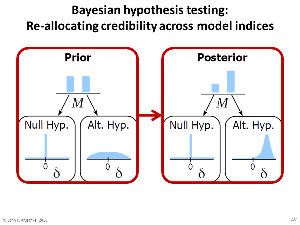
Bayesian hypothesis testing: Suppose we are modeling some data with a model that has parameter δ in which we are currently interested, along with some other parameters. A null hypothesis model can be formulated as a prior on the parameters that puts a "spike" at the null value of δ but is spread out over the other parameters. A non-null alternative model puts a prior on δ that allows non-null values. The two models are indexed by a higher-level discrete parameter M. The entire hierarchy (a mixture model) has all its parameters updated by the data. The following slide from my workshops illustrates:


The Bayes factor (BF) is the shift in model-index probabilities:


Digression: I throw in two usual caveats about using Bayes factors. First, Bayesian model comparison --for null hypothesis testing or more generally for any (non-nested) models-- must use meaningful priors on the parameters in both models for the Bayes factor to be meaningful. Default priors for either model are typically not very meaningful and quite possibly misleading.
And, the Bayes factor is not the posterior probability of the models. Typically we ultimately want to know the posterior probabilities of the models, and the BF is just a step in that direction.
Link in slide above: http://doingbayesiandataanalysis.blogspot.com/2015/12/lessons-from-bayesian-disease-diagnosis_27.html

Assessing null value through parameter estimation: There's another way to assess null values. This other way focuses on the (marginal) posterior distribution of the parameter in which we're interested. (As mentioned at the outset, this approach is not called "hypothesis testing.") This approach is analogous to frequentist equivalence testing, which sets up a region of practical equivalence (ROPE) around the null value of the parameter:
 
The logic of this approach stems from a direct reading of the meaning of the intervals. We decide to reject the null value when the 95% highest density parameter values are all not practically equivalent to the null value. We decide to accept the null value when the 95% highest density parameter values are all practically equivalent to the null value. Furthermore, we can make direct probability statements about the probability mass inside the ROPE such as, "the probability that the parameter is practically equivalent to the null is 0.017" or "the probability that the parameter is practically equivalent to the null is 0.984."

The ROPE is part of the decision rule, not part of the null hypothesis. The ROPE does not constitute an interval null hypothesis; the null hypothesis here is a point value. The ROPE is part of the decision rule for two main purposes: First, it allows decisions to accept the null (again, analogous to frequentist equivalence testing). Second, it makes the decision rule asymptotically correct: As data sample size increases, the rule will come to the correct decision, either practically equivalent to the null value (within the ROPE) or not (outside the ROPE).

Juxtaposing the two approaches: Notice that the two approaches to assessing null values are not equivalent and have different emphases. The BF focuses on the model index, whereas the HDI and ROPE focus on the parameter estimate:


Therefore the two approaches will not always come to the same decision, though often they will. Neither approach is uniquely "correct;" the two approaches frame the question differently and provide different information. 

Below is an example of the different information provided by hypothesis testing and estimation (for both frequentist and Bayesian analyses). The data are dichotomous, with z=14 successes out N=18 attempts (e.g., 14 heads out of 18 flips). The data are modeled by a Bernoulli distribution with parameter θ. The null value is taken to be θ=0.50. For the Bayesian analysis, the alternative-hypothesis prior is uniform merely for purposes of illustration; uniform is equivalent to dbeta(1,1).
From: Kruschke, J. K. and Liddell, T. (in press 2016), The Bayesian New Statistics: Hypothesis testing, estimation, meta-analysis, and power analysis from a Bayesian perspective. Psychonomic Bulletin & Review.
You can see above that Bayesian hypothesis testing and Bayesian parameter estimation provide very different information. Which approach to use for assessing the null value then comes down to careful interpretation and practicalities. For more discussion please see this article: Kruschke, J. K. and Liddell, T. (2017), The Bayesian New Statistics: Hypothesis testing, estimation, meta-analysis, and power analysis from a Bayesian perspective. Psychonomic Bulletin & Review.

Friday, December 16, 2016

The Bayesian New Statistics: Hypothesis Testing, Estimation, Meta-Analysis, and Power Analysis from a Bayesian Perspective

UPDATE: Now published, see this post.

Two conceptual distinctions in the practice of data analysis. Rows show point-value hypothesis testing versus estimating magnitude with uncertainty. Columns show frequentist versus Bayesian methods. Cells indicate the typical information provided by each approach. [Figure 1 of Kruschke & Liddell (in press), The Bayesian new statistics: Hypothesis testing, estimation, meta-analysis, and power analysis from a Bayesian perspective. Psychonomic Bulletin & Review.]
Many people have found the table above to be useful for understanding two conceptual distinctions in the practice of data analysis. The article that discusses the table, and many other issues, is now in press. (It was submitted in mid May, 2015, and was just accepted; a blog post announcing its original version is here, along with many comments.) The in-press version can be found at OSF and at SSRN.

Abstract: In the practice of data analysis, there is a conceptual distinction between hypothesis testing, on the one hand, and estimation with quantified uncertainty, on the other hand. Among frequentists in psychology a shift of emphasis from hypothesis testing to estimation has been dubbed "the New Statistics" (Cumming, 2014). A second conceptual distinction is between frequentist methods and Bayesian methods. Our main goal in this article is to explain how Bayesian methods achieve the goals of the New Statistics better than frequentist methods. The article reviews frequentist and Bayesian approaches to hypothesis testing and to estimation with confidence or credible intervals. The article also describes Bayesian approaches to meta-analysis, randomized controlled trials, and power analysis.

Wednesday, November 16, 2016

Is it legitimate to view the data and then decide on a distribution for the dependent variable?

An emailer asks,
In Bayesian parameter estimation, is it legitimate to view the data and then decide on a distribution for the dependent variable? I have heard that this is not “fully Bayesian”.
The shortest questions often probe some of the most difficult issues; this is one of those questions.

Let me try to fill in some details of what this questioner may have in mind. First, some examples:
  • Suppose we have some response-time data. Is it okay to look at the response-time data, notice they are very skewed, and therefore model them with, say, a Weibull distribution? Or must we stick with a normal distribution because that was the mindless default distribution we might have used before looking at the data? Or, having noticed the skew in the data and decided to use a skewed model, must we now obtain a completely new data set for the analysis?
  • As another example, is it okay to look at a scatter plot of population-by-time data, notice they have a non-linear trend, and therefore model them with, say, an exponential growth trend? Or must we stick with a linear trend because that was the mindless default trend we might have used before looking at the data? Or, having noticed the non-linear trend in the data and decided to use a non-linear model, must we now obtain a completely new data set for the analysis?
  • As a third example, suppose I’m looking at data about the positions of planets and asteroids against the background of stars. I’m trying to fit a Ptolemaic model with lots of epicycles. After considering the data for a long time, I realize that a completely different model, involving elliptical orbits with the sun at a focus, would describe the data nicely. Must I stick with the Ptolemaic model because it’s what I had in mind at first? Or, having noticed the Keplerian trend in the data, must I now obtain a completely new data set for the analysis?
What is the worry of the unnamed person who said it would not be “fully Bayesian” to look at the data and then decide on the model? I can think of a few possible worries:

One worry might be that selecting a model after considering the data is HARKing (hypothesizing after the results are known; Kerr 1998, http://psr.sagepub.com/content/2/3/196.short). Kerr even discusses Bayesian treatments of HARKing (pp. 206-207), but this is not a uniquely Bayesian problem. In that famous article, Kerr discusses why HARKing may be inadvisable. In particular, HARKing can transform Type I errors (false alarms) into confirmed hypothesis ergo fact. With respect to the three examples above, the skew in the RT data might be a random fluke, the non-linear trend in the population data might be a random fluke, and the better fit by the solar-centric ellipse might be a random fluke. Well, the only cure to Type I errors (false alarms) is replications (as Kerr mentions). Pre-registered replications. There are lots of disincentives to replication attempts, but these disincentives are gradually being mitigated by recent innovations like registered replication reports (https://www.psychologicalscience.org/publications/replication). In the three examples above, there are lots of known replications of skewed RT distributions, exponential growth curves, and elliptical orbits.

Another worry might be that the analyst had a tacit but strong theoretical commitment to a particular model before collecting the data, and then reneged on that commitment by sneaking a peak at the data. With respect to the three examples above, it may have been the case that the researcher had a strong theoretical commitment to normally distributed data, but, having noticed the skew, failed to mention that theoretical commitment and used a skewed distribution instead. And analogously for the other examples. But I think this mischaracterizes the usual situation of generic data analysis. The usual situation is that the analyst has no strong commitment to a particular model and is trying to get a reasonable summary description of the data. To be “fully Bayesian” in this situation, the analyst should set up a vast model space that includes all sorts of plausible descriptive models, including many different noise distributions and many different trends, because this would more accurately capture the prior uncertainty of the analyst than a prior with only a single default model. But doing that would be very difficult in practice, as the space of possible models is infinite. Instead, we start with some small model space, and refine the model as needed.

Bayesian analysis is always conditional on the assumed model space. Often the assumed model space is merely a convenient default. The default is convenient because it is familiar to both the analyst and the audience of the analysis, but the default need not be a theoretical commitment. There are also different goals for data analysis: Describing the one set of data in hand, and generalizing to the population from which the data were sampled. Various methods for penalizing overfitting of noise are aimed at finding a statistical compromise between describing the data in hand and generalizing to other data. Ultimately, I think it only gets resolved by (pre-registered) replication.

This is a big issue over which much ink has been spilled, and the above remarks are only a few off-the-cuff thoughts. What do you think is a good answer to the emailer's question?

Thursday, November 3, 2016

Bayesian meta-analysis of two proportions in random control trials


For an article that's accepted pending final revision (available here at OSF), I developed a Bayesian meta-analysis of two proportions in random control trials. This blog post summarizes and links to the complete R scripts.

We consider scenarios in which the data consist of the number of occurrences and the number of opportunities in a control group and in a treatment group.  The number of occurrences in the treatment group is denoted \(z_T\) and the number of opportunities in the treatment group is denoted \(n_T\), and analogously \(z_C\) and \(n_C\) in control group. The proportion of occurrences in the treatment group is \(z_T/n_T\), and the proportion of occurrences in the control group is \(z_C/n_C\).

For example, perhaps we are interested in the occurrence of mortality after myocardial infarction (death after heart attack), in a control group and in a group treated with beta-blockers (heart muscle relaxant). In this case, if beta-blockers have a beneficial effect, \(z_T/n_T\) should be less than \(z_C/n_C\).

As another example, perhaps we are interested in re-use of towels by patrons of hotels (instead of having towels changed every day for the same patron, which wastes laundering electricity and detergent). We consider towel re-use in a control group and in a group treated with a sign that indicates it's normal for people to re-use their towels. In this case, if the treatment has a beneficial effect, \(z_T/n_T\) should be greater than \(z_C/n_C\).


In meta-analysis, there are several studies that each test the treatment. The data from study \(s\) are denoted \(z_{T[s]}, n_{T[s]}, z_{C[s]}, n_{C[s]}\). Each study is conducted at its own site (e.g., hotel, hospital). Because each site has its own specific attributes, we do not expect the underlying proportions of occurrence to be identical across sites. But we do expect them to be similar and mutually informative, so we treat the data from different sites as representative of higher-level parameters in the model that describe what's typical across sites and how much variability there is across sites. This approach is the usual random-effects model for meta-analysis.

Here are the parameters I'll use to describe the data:
  • \(\theta_{C[s]}\) is the probability of occurrence in the control group for study \(s\).
  • \(\theta_{T[s]}\) is the probability of occurrence in the treatment group for study \(s\).
  • \(\rho_{[s]}\) is the difference of log-odds between groups:
       \(\rho_{[s]} = logit(\theta_{T[s]}) - logit(\theta_{C[s]})\)
Re-arranged, the equation for \(\rho_{[s]}\) expresses the relation of \(\theta_{T[s]}\) to \(\theta_{C[s]}\): \[ \theta_{T[s]} = logistic( \rho_{[s]} + logit( \theta_{C[s]} ) )\] This relation is a natural way to represent the dependency of the probabilities between groups because the relation is (i) symmetric with respect to what outcome is defined as success or failure because \(logit(\theta) = -logit(1-\theta)\), and (ii) symmetric with respect to which group is defined as the treatment by reversing the sign of \(\rho\). Note that \(\rho_{[s]}\) is the so-called log odds ratio across groups: \(\rho_{[s]} = log( [\theta_{T[s]}/(1-\theta_{T[s]})] / [\theta_{C[s]}/(1-\theta_{C[s]})] )\). I hope this little explanation and motivation of \(\rho_{[s]}\) is helpful.

I'll describe the distribution of  \(\theta_{C[s]}\) across studies as a beta distribution, parameterized by its mode and concentration:
  • \(\omega_{\theta C}\) is the modal value (of the beta description) of \(\theta_{C[s]}\)
  • \(\kappa_{\theta C}\) is the concentration (of the beta description) of \(\theta_{C[s]}\)
For beta distributions parameterized by the usual \(a,b\) shape parameters, we convert mode and concentration to \(a,b\), and the above specification becomes \(\theta_{C[s]} \sim beta( \omega_{\theta C}(\kappa_{\theta C}-2)+1 , (1-\omega_{\theta C})(\kappa_{\theta C}-2)+1 )\).

I'll describe the distribution of  \(\rho_{[s]}\) across studies as a normal distribution, parameterized by its mean and standard deviation:
  • \(\mu_{\rho}\) is the mean (of the normal description) of \(\rho_{[s]}\)
  • \(\sigma_{\rho}\) is the standard deviation (of the normal description) of \(\rho_{[s]}\) 
In other words, for a normal distribution parameterized by mean and precision as in JAGS, \( \rho_{[s]} \sim normal( \mu_{\rho} , 1/\sigma_{\rho}^2 ) \). Usually, the primary focus of research is the value of \(\mu_{\rho}\), that is, the estimate of the treatment effect across studies.

This type of hierarchical model is a typical random-effects model for meta-analysis, because the model gives each study its own individual parameter values which are assumed to be ("exchangably") representative of a common underlying tendency.

I'll set vague priors on the top-level parameters. An implementation of the model in R, JAGS, and runjags is provided below.

Notice that an alternative model that estimated \(\theta_{C[s]}\) independently from \(\theta_{T[s]}\), and then computed \(\rho_{[s]}\) afterwards, would not produce the same results. Nor would it be an appropriate model! It would not be appropriate because it would treat the control group and treatment group in the same study as being completely unrelated --- if we independently permuted the study indices in the treatment and control groups (i.e., re-arranged which control groups go with which treatment groups) the results of this alternative model would be unchanged. Instead, the model I am using assumes that the treatment probability is linked to the control probability. For example, if one  hospital has a low rate of heart attacks in the control condition but another hospital has a high rate of heart attacks in the control condition, the treatment should reduce heart attacks relative to the particular hospital's base rate, not to some absolute rate independent of hospital.


I'll apply the model to two sets of data. First, some data on death after heart attack, summarized on pp. 124-128 of Gelman et al., 2014, Bayesian Data Analysis, Third Edition. There were 22 studies, involving as few as 77 patients and as many as 3,887 patients. The treatment group received beta-blockers. If the treatment is effective, the log-odds-ratio will be less than 0. Below is a forest plot of the results:

In the plot above, each of the 22 lower rows shows an individual study's observed log-odds-ratio with a gray triangle. Notice that the gray triangle is greater than 0 in 6 of the 22 studies. The size of the triangle indicates the sample size in the study. The blue distribution is the posterior distribution for \(\rho_{[s]}\). The distribution is marked with its modal value and its 95% highest density interval (HDI). The numerical values of the mode and HDI are indicated at the right margin. At the top of the plot is shown the posterior distribution of \(\mu_{\rho}\). In words, this means that across studies the typical effect of treatment has a log-odds-ratio of about \(-0.25\), with a range of uncertainty from \(-0.39\) to \(-0.12\), well below 0. (These values are very similar to those reported by Gelman et al., BDA3, Table 5.3, p. 127.)

Notice also in the forest plot above that there is strong shrinkage of the individual study estimates toward the modal value across studies. For example, Study 22 has a greatly reduced rate of heart attack in its treatment group (gray triangle is at a low value), but the posterior estimate of its treatment effect is not so extreme, and its posterior distribution shows a skew to accommodate the "pull" of the extreme data from the shrunken distribution. Complementary skew and shrinkage can be seen, for example, in Study 14. The posterior distributions of the individual studies also show different uncertainties depending on the sample size in the study. For example, Study 10, with a large sample size, has a much narrower HDI than Study 19 with its small sample size.

Here is another application. In this case the data come from studies of towel re-use (Scheibehenne, Jamil, and Wagenmakers (2016). Bayesian evidence synthesis can reconcile seemingly inconsistent results: The case of hotel towel reuse. Psychological Science, 27, 1043-1046). At 7 different hotels, patrons in the treatment group were told it is normal to re-use towels (see article for details). If the treatment is effective, the log-odds-ratio should be greater than 0. Here is a forest plot of the results from the analysis:
(In Study 1 above, the gray triangle is so small that it falls outside of the plot range. It had N=162.) In this case, because there were only 7 studies and wide variation in the results across studies, the overall estimate of the log-odds-ratio is fairly uncertain: Its 95% HDI goes from \(-0.12\) to \(+0.47\). While the mode of the overall estimate is positive (at \(0.21\)), the uncertainty is great enough that we would want to do more studies to nail down the magnitude of the effect of treatment. Notice also the posterior distributions of the individual studies: There is evident shrinkage, but also lots of uncertainty, again with smaller studies showing more uncertainty than larger studies.

(In Scheibehenne et al.'s published analysis, a fixed-effects model was used, which is tantamount to using a single \(\rho\) and single \(\theta_C\) for all studies. This can be approximated in the model used here by specifying a prior that forces there to be tiny variance across \(\rho_{[s]}\) and tiny variance across \(\theta_{C[s]}\).)

As mentioned at the beginning, this model was developed for an article that is accepted pending final revision, available here. I also talked about Bayesian meta-analysis, and these applications in particular, in a presentation about Bayesian methods for replication analysis, that you can watch here.

The complete R script is available here.